The size and persistence of inflation post-COVID-19 was among the largest problems the U.S. economy has faced in decades. The rise in house prices was a major contributor to this inflationary episode. Understanding this housing boom is critical for policymakers to connect the consequences of their actions, particularly as it relates to the relationship between inflation and quantitative easing (QE). This paper examines the impact of quantitative easing undertaken by the Federal Reserve from 2020 to 2022, during which the Fed’s mortgage-backed securities (MBS) purchases ($1.33 trillion) were equal to nearly 90% of the growth in MBS ($1.50 trillion). Evidence suggests that housing’s unique role as an asset class is a factor explaining the rise in the cost of housing and hence overall inflation. Should this be the case, the Federal Reserve should reconsider the impact of future quantitative easing on housing values and, subsequently, shelter inflation.
COVID-19 shocked the global economy, causing a severe recession. Monetary and fiscal policy activated to support the economy and later transitioned to fighting inflation after the recovery. In the initial period following the onset of the pandemic, the Federal Reserve’s (Fed) monetary policy response was to cut interest rates to the zero lower bound, activate a series of emergency lending facilities to support a wide array of financial assets, and engage in quantitative easing (QE). Post-recession the Fed began raising interest rates, ended its emergency lending facilities, and stopped QE. The recovery from the COVID pandemic brought the highest inflation the U.S. has seen in decades; annual growth of the Consumer Price Index (CPI) reached 9% in 2022. Economists continue to debate the causes of this inflationary episode.
COVID supply shocks, unprecedented fiscal stimulus, and rapidly shifting consumption preferences have all received substantial attention as underlying factors triggering inflation. At the Fed’s 2024 Jackson Hole Economic Symposium, Federal Reserve Chairman Jerome Powell gave a list of reasons for inflation in the U.S.: “supply chain shocks, speed of demand snap-back post-pandemic, Russia’s invasion of Ukraine, and tight labor markets.” Housing was absent altogether from his list. However, the path of housing inflation differed from overall inflation and remains elevated while other categories have cooled.
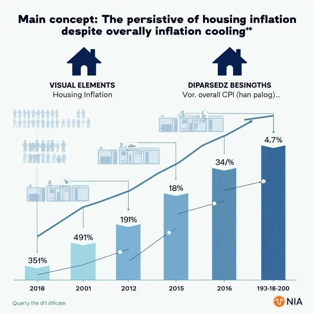
As shown in Figure 1, before COVID, housing inflation had been stable and above overall CPI. During the inflation spike in 2021, housing inflation remained low initially, falling below overall inflation for the first time in almost a decade. After overall inflation took off, housing inflation followed. While overall inflation peaked in mid-2022, housing inflation kept rising, peaking almost a full year later in early 2023. Subsequently, while overall inflation has eased, housing inflation remains elevated at an annual change of 5% in mid-2024 and 4% in mid-2025, whereas overall CPI is down to 3% and non-housing inflation is down to 2%. The persistence of housing inflation is a leading factor in the persistence of overall inflation above the 2% target even long after other sectors have cooled.
La inflación del costo de la vivienda es central en el episodio inflacionario de América. La vivienda es la mayor inversión para la mayoría de las familias y representa el 45% del IPC. La vivienda comprende muchos sub-elementos del IPC, incluidos los elementos involucrados en el costo de mantener una casa (muebles, seguro, electrodomésticos, el costo de vivir fuera de casa, etc.). Este papel se centra en el costo de la casa misma, ya sea el valor de la propiedad para un propietario o el costo del alquiler para un inquilino. Estos forman la mayor parte de la vivienda, como se esperaba. El albergue, el término utilizado por el IPC para esto, es el 36% del IPC total y es igual al 80% del elemento general dentro de la vivienda. El albergue incluye el alquiler equivalente de la propiedad de un propietario, la métrica que utiliza el IPC para evaluar el valor de la casa de un propietario (si fuera alquilarla) que solo es más de un cuarto del IPC total. También incluye el alquiler de inquilinos que comprende el 7,7% del IPC total. Que el alquiler de inquilinos es una parte menor del IPC total refleja que solo un tercio de los estadounidenses son inquilinos, mientras que dos tercios viven en una casa que ellos o su familia poseen. El papel se centra principalmente en el impacto de los precios de las casas, central para el alquiler equivalente de la propiedad. Este valor también puede impactar el costo de alquilar vivienda. Además, la consideración de la inflación de la vivienda en la política se complica por el hecho de que las proyecciones de inflación del Fed han estado equivocadas en la inflación de la vivienda. En agosto de 2023, el Banco de la Reserva Federal de San Francisco proyectó que la inflación del albergue era “probablemente disminuir”, prediciendo una disminución constante de la inflación del albergue alcanzando un crecimiento del 0% en mitad de 2024. En cambio, la inflación del albergue permaneció elevada, aumentando un 5% anual en mitad de 2024 y un 4% en mitad de 2025. Si la inflación real del albergue hubiera seguido las proyecciones del Banco de la Reserva Federal de San Francisco, el crecimiento del IPC total habría estado por debajo del objetivo del 2% del Fed en 2024, en lugar de estar por encima de él. Dado que el Fed decidió mantener las tasas de interés elevadas hasta septiembre de 2024 debido a la inflación persistente, es posible que el Federal Reserve hubiera comenzado a reducir las tasas de interés meses antes si la inflación de la vivienda hubiera disminuido como el Fed proyectó o incluso a la misma velocidad y ritmo que el resto de la economía. Este papel examina el papel del Federal Reserve en la inflación de la vivienda enfocándose en el impacto de la QE. El programa de QE del Fed consistió en grandes compras de bonos del Tesoro y títulos hipotecarios (MBS) con el propósito de reducir aún más las tasas de interés después de que la tasa de fondos federales hubiera alcanzado el límite inferior cero. La tesis es que las grandes compras del Fed de MBS, implementadas como parte de la QE desde 2020 hasta 2022, contribuyeron a la apreciación de los precios de las casas, causando parte de la inflación de la vivienda que el Fed posteriormente aumentó las tasas de interés para combatir. Si bien las tasas de interés más altas debilitan la demanda, las tasas de interés aumentadas tuvieron un efecto limitado en la inflación de la vivienda debido a la rigidez de precios descendente en el mercado de la vivienda. Si es correcto, el Fed necesita reconsiderar su plan de acción cuando la política monetaria alcanza el límite inferior, específicamente para considerar los impactos de precios de los activos que compra. Este papel está organizado de la siguiente manera: La sección dos discute la teoría de cómo y por qué la QE tendría un impacto en los precios de las casas. La sección tres examina el impacto de la QE en el mercado de la vivienda desde marzo de 2020 hasta marzo de 2022 y los efectos en juego después de la QE desde marzo de 2022 en adelante. El papel concluye con una sección que examina explicaciones alternativas para los cambios vistos en el mercado de la vivienda.
El papel del Federal Reserve en la inflación de la vivienda
El papel del Federal Reserve en la inflación de la vivienda es un tema complejo que requiere una comprensión profunda de la economía y la política monetaria. El Federal Reserve tiene el poder de influir en la economía a través de la política monetaria, y su papel en la inflación de la vivienda es un aspecto crucial de su función. El papel de este artículo es examinar el papel del Federal Reserve en la inflación de la vivienda, enfocándose en el impacto de la QE. El programa de QE del Fed consistió en grandes compras de bonos del Tesoro y títulos hipotecarios (MBS) con el propósito de reducir aún más las tasas de interés después de que la tasa de fondos federales hubiera alcanzado el límite inferior cero. La tesis es que las grandes compras del Fed de MBS, implementadas como parte de la QE desde 2020 hasta 2022, contribuyeron a la apreciación de los precios de las casas, causando parte de la inflación de la vivienda que el Fed posteriormente aumentó las tasas de interés para combatir.
Impacto de la QE en el mercado de la vivienda
El impacto de la QE en el mercado de la vivienda es un tema crucial que requiere una comprensión profunda de la economía y la política monetaria. El programa de QE del Fed consistió en grandes compras de bonos del Tesoro y títulos hipotecarios (MBS) con el propósito de reducir aún más las tasas de interés después de que la tasa de fondos federales hubiera alcanzado el límite inferior cero. La tesis es que las grandes compras del Fed de MBS, implementadas como parte de la QE desde 2020 hasta 2022, contribuyeron a la apreciación de los precios de las casas, causando parte de la inflación de la vivienda que el Fed posteriormente aumentó las tasas de interés para combatir. El impacto de la QE en el mercado de la vivienda es un tema complejo que requiere una comprensión profunda de la economía y la política monetaria.
Conclusión
En conclusión, el papel del Federal Reserve en la inflación de la vivienda es un tema complejo que requiere una comprensión profunda de la economía y la política monetaria. El papel de este artículo es examinar el papel del Federal Reserve en la inflación de la vivienda, enfocándose en el impacto de la QE. El programa de QE del Fed consistió en grandes compras de bonos del Tesoro y títulos hipotecarios (MBS) con el propósito de reducir aún más las tasas de interés después de que la tasa de fondos federales hubiera alcanzado el límite inferior cero. La tesis es que las grandes compras del Fed de MBS, implementadas como parte de la QE desde 2020 hasta 2022, contribuyeron a la apreciación de los precios de las casas, causando parte de la inflación de la vivienda que el Fed posteriormente aumentó las tasas de interés para combatir.
El Quantitative Easing (QE) es la compra de activos en el mercado abierto por parte de la Reserva Federal. El QE comenzó como una respuesta teórica a las preguntas de qué podría hacer una banca central si se encontraba atrapada por el llamado “límite inferior cero” de la política de tipos de interés (establecer tipos de interés en cero). La Reserva Federal se enfrentó a este dilema después de la crisis financiera global de 2008 (GFC). El epicentro de la GFC fue el sistema de financiamiento de la vivienda en Estados Unidos, con una combinación de préstamos hipotecarios mal avalados y altamente endeudados que llevaron a una explosión y una quiebra de la vivienda estadounidense. Como parte de la respuesta a la GFC, la Reserva Federal inició el QE en noviembre de 2008. La Reserva Federal está limitada por ley en cuanto a qué activos puede comprar para implementar el QE. La Sección 14 de la Ley de la Reserva Federal prescribe los activos que la Reserva Federal puede comprar: obligaciones directas del Tesoro de los Estados Unidos (Tesoros) y obligaciones garantizadas por empresas patrocinadas por el gobierno (GSEs). En la práctica, los únicos títulos de GSE que pueden ser adquiridos por la Reserva Federal son los títulos hipotecarios respaldados por Fannie Mae, Freddie Mac o Ginnie Mae. Estas tres empresas compran, garantizan y securitan la mayoría de los préstamos hipotecarios en Estados Unidos, y su deuda de títulos hipotecarios respaldados es a menudo referida como “títulos hipotecarios respaldados por agencias”. Las restricciones legales de la Reserva Federal para comprar títulos del Tesoro y deuda hipotecaria resultan en que estos dos activos sean el método a través del cual se implementa el QE. El mercado de deuda del Tesoro alcanzó los $36 billones mientras que el mercado de deuda hipotecaria supera los $9 billones. Como resultado de las dos rondas de QE, la Reserva Federal es ahora un importante poseedor de ambos activos. En su punto máximo en mitad de 2022, la Reserva Federal poseía casi un quinto de todos los títulos del Tesoro y más de un cuarto de los títulos hipotecarios respaldados por agencias. El QE duró hasta marzo de 2022 cuando la Reserva Federal dejó de comprar nuevos títulos. La Reserva Federal mantuvo sus holdings de títulos hipotecarios respaldados por agencias constantes (comprando nuevos para compensar el desglose existente) durante tres meses. A partir de junio de 2022, la Reserva Federal ha estado permitiendo que su cartera se desglose naturalmente. Algunos llaman a la desaceleración gradual del QE “tensión cuantitativa” (QT). Sin embargo, hay una diferencia entre permitir que los holdings de títulos hipotecarios respaldados por agencias se desglosen naturalmente (comprando nuevos para compensar el desglose existente) y la Reserva Federal vendiendo títulos hipotecarios respaldados por agencias al mercado. La Reserva Federal: El mayor jugador en el mercado de la vivienda ¿Cuán grande fue la compra de la Reserva Federal en este mercado? La propiedad de la Reserva Federal de $2.7 billones de títulos hipotecarios respaldados por agencias en 2022 era del 32% del mercado de títulos hipotecarios respaldados por agencias completo de $8.5 billones. Durante el período de QE de 2020-2022, el mercado de títulos hipotecarios respaldados por agencias aumentó en $1.50 billones, de los cuales la Reserva Federal compró $1.33 billones. Las compras de la Reserva Federal de títulos hipotecarios respaldados por agencias fueron iguales a casi el 90 por ciento del crecimiento en el mercado de títulos hipotecarios respaldados por agencias durante el período de QE. El mercado de títulos hipotecarios respaldados por agencias no es el mercado de la vivienda completo. Se centra principalmente en casas de una sola familia (definidas como una a cuatro unidades) que requieren un préstamo. Esto excluye las casas compradas con todo el dinero, que ha sido alrededor de un tercio de las casas compradas desde la pandemia. No incluye los préstamos hipotecarios hechos que no eran elegibles para títulos hipotecarios respaldados por agencias (jumbo, grandes porciones de bienes raíces comerciales no enviados a través de las GSEs, préstamos hipotecarios mantenidos por bancos). Sin embargo, los títulos hipotecarios respaldados por agencias apoyan la mayor parte de los préstamos hipotecarios. Los préstamos hipotecarios respaldados por Fannie Mae, Freddie Mac y Ginnie Mae juntos representan más del 65 por ciento de los préstamos hipotecarios totales. Además, estos préstamos hipotecarios respaldados por agencias representan casi la totalidad de los compradores de viviendas por primera vez que están pasando de ser inquilinos a compradores de viviendas o dejando una unidad de vivienda familiar anterior para empezar una nueva. Los compradores de viviendas por primera vez representaron el 32 por ciento de las ventas de viviendas en 2022, mostrando su importancia para impulsar el mercado de compras de viviendas. Los títulos hipotecarios respaldados por agencias también son un componente importante para la vivienda de alquiler. Si bien muchos inquilinos están en edificios de apartamentos grandes, alrededor de la mitad de las unidades de alquiler son casas de una a cuatro unidades. ¿Cómo el QE impacta los precios de la vivienda? El canal para el impacto del QE en los precios de la vivienda es el siguiente. La demanda de la Reserva Federal de títulos hipotecarios respaldados por agencias aumenta el valor de los préstamos hipotecarios. La incentivación para crear préstamos hipotecarios resulta en tipos de interés hipotecarios más bajos, lo que induce a las personas a comprar o refinanciar. Los tipos de interés hipotecarios más bajos también aumentan la demanda de vivienda ya que la propiedad de una vivienda se vuelve más asequible. Las leyes básicas de la oferta y la demanda llevan a la suposición de que un gran aumento en la demanda impactará el precio y la cantidad. Los impactos en el precio se magnifican cuando la cantidad está fija en el corto plazo. La vivienda tiene una capacidad limitada para ajustar la oferta en el corto plazo; le toma tiempo construir una casa y algunos mercados están limitados debido a la regulación o no tener suficiente tierra. Esto sugiere impactos en los precios de la vivienda en el corto plazo. El ex presidente de la Reserva Federal, Ben Bernanke, reconoció el impacto de las compras de títulos hipotecarios respaldados por agencias en los rendimientos, afirmando: Las compras de la Reserva Federal de títulos hipotecarios respaldados por agencias, por ejemplo, deberían aumentar los precios y reducir los rendimientos de esos títulos; además, como los inversores rebalancean sus carteras reemplazando los títulos hipotecarios respaldados por agencias vendidos a la Reserva Federal con otros activos, los precios de los activos que compran deberían aumentar y sus rendimientos deberían disminuir también. Los rendimientos decrecientes y los precios aumentados facilitan las condiciones financieras generales y estimulan la actividad económica a través de canales similares a los de la política monetaria convencional. Las acciones de rebalanceo de los inversores deberían extender el descenso de rendimientos a través de otros activos. Sin embargo, si bien las diferencias de tipos de interés hipotecarios disminuyeron durante el QE, aumentaron después del QE, lo que sugiere que las compras de títulos hipotecarios respaldados por agencias durante el QE comprimieron los tipos de interés hipotecarios más que los rendimientos de otros activos similares calificados, como los bonos corporativos AAA. Las acciones de rebalanceo pueden no haber podido extender uniformemente el impacto del QE a través de otros activos debido a que la Reserva Federal compró casi el 90 por ciento del crecimiento en el mercado de títulos hipotecarios respaldados por agencias durante este período. Un estudio publicado por la Reserva Federal de Kansas City corrobora estos hallazgos afirmando, “Un aumento de 10 puntos porcentuales en la participación
Starting in 2020, the housing market deviated from its pre-pandemic path. Three key trends which shifted in 2020 after QE began and in 2022 after QE ended are identified: Housing values soared during QE and plateaued after. Home sales increased sharply during QE and dropped after. There was a wave of refinancing during QE. These three trends are correlated with the Fed’s MBS purchases, and there is a causal relationship as will be explored. This section then discusses the impact of MBS purchases on the housing market and the broader economy through housing wealth effects. Additionally, effects at play in the housing market after the end of QE in 2022 (interest rate lock-in, home equity and loss aversion effects) and their role in maintaining plateaued house prices and sparse home sales are considered.
Housing values soared from 2020 to 2022: The average value of a house rose by nearly $100,000. This asset value explosion marks a sudden shift from pre-pandemic trends of slow and steady appreciation between 2012 and 2020. The average/median home in America rose by around $12,300 per year (nominally) during the period between the GFC and COVID-19-equal to 6% growth per year on average. From Q2 2020 to Q2 2022, the average/median home value grew by around $100,000 ($95,800 is the exact estimate), which translates to an asset value increase of nearly 17% per year on average. Less than one-quarter of that growth ($21,500) would be expected had housing followed its pre-pandemic growth pattern. About three-quarters of that growth ($74,300) is greater than the trendline of home price appreciation would have predicted. The increase in home values can be seen both in statistical imputations of home values and observed sales prices.
Home sales plunged during the pandemic, increased sharply during QE, then dropped to pandemic lows after QE, as shown by Figure 7. COVID-19 caused the housing market to freeze. Shutdowns and restrictions resulted in the inability for many house sales and purchases to occur. The housing market returned as workarounds were found and restrictions lifted. Home sale volumes then rebounded to historic highs as restrictions were lifted further and the Fed loosened monetary policy. After QE ended in March 2022, home sales declined to 100,000 sales per month lower than the pre-pandemic average.
A massive wave of refinancing occurred during the QE period. More than three-quarters of all GSE mortgages originated in 2021 were refinances. Approximately one-third of outstanding mortgage balances was refinanced during the seven quarters of the refi boom, and an additional 17% of mortgages outstanding were refreshed through home sales during a time of high demand for housing. Many homeowners extracted their home equity as cash through cash-out refinances. A total of $430 billion was cashed out.
QE and the housing market
The sharp appreciation in home values occurred during the period of the Fed’s QE. Overlaying the Fed’s balance sheet and home values, the correlation is clear. Going into COVID, the Fed had been slowly shrinking the MBS it acquired during the previous round of QE after the GFC. The Fed lowered its holdings to around $1.4 trillion of MBS when the COVID recession hit. The Fed announced QE on March 15, 2020, committing to “increase its holdings of Treasury securities by at least $500 billion and its holdings of agency mortgage-backed securities by at least $200 billion.” The final amount of purchases far exceeded the initial numbers. The Fed purchased $1.3 trillion of agency MBS from March 2020 to March 2022. Their total ownership at peak was $2.7 trillion, 32% of the entire $8.5 trillion MBS market. During this period, total agency MBS increased by $1.50 trillion, of which the Fed’s MBS purchases were equal to nearly 90% of the increase in MBS during the QE period.
The correlation between the Fed’s MBS purchases and house price appreciation is clear. Causation is difficult to prove with multiple factors involved, though the tightening of spreads between mortgages and other assets, insights from the GFC, and expansion of the agency MBS market support the connection between the Fed’s purchases of MBS and house price appreciation. Economic logic also suggests that a QE strategy confined to mortgages, which results in the central bank being the dominant buyer of mortgage MBS, will have a disproportionate impact on home prices. Increased home values have an impact on aggregate demand and inflation through the wealth channel. Estimates suggest this provided at least $400 billion of additional stimulus to the economy. However, it also increased inflation as observed in housing inflation.
Interest rate lock-in effect
Existing homeowners who refinanced during the pandemic were able to capture generationally low interest rates. The Fed’s subsequent sharp rise in interest rates means that an existing homeowner needing a new mortgage will likely receive a substantially higher interest rate. This creates an interest rate lock-in effect where existing homeowners are less likely to move as they would lose their lower interest rate mortgage in the process. It is possible that sharp house price appreciation during QE intensified the interest rate lock-in effect after QE since mortgage payments increase more for higher priced homes. For example, an increase in mortgage rates from 3 to 6% increases the mortgage payment on a $200,000 house by $356 per month and increases the payment on a $300,000 house by $534 per month.
The constraint on mobility created by the interest rate lock-in effect impacts house price in both directions. On one hand, higher mortgage rates freeze the housing market and decrease the supply of homes for sale, applying upward pressure. On the other hand, higher mortgage rates reduce housing demand as households’ budgets are constrained to afford smaller mortgages and “locked” households do not enter the market, applying downward pressure. The net effect on price depends on whether lock-in blocks more downsizing than upsizing. The Federal Housing Finance Agency studied this exact issue and concluded that from 2022 Q2 to 2024 Q2, interest rate lock-in led to a 1.7 million decrease in home sales which increased prices by 7.0%, outweighing what the paper estimated as the 5.6% decrease in home prices from high interest rates. The net effect of interest rate lock-in was a 1.4% price increase.
Home equity and nominal loss aversion
Next, how low or negative home equity constrains homeowner mobility is examined. This has been modeled by assuming existing homeowners rely on their home equity to fund their downpayment for another house, assuming they do not have an extra source of wealth and prefer to continue owning. Thus, prospective sellers need to sell at a price where their profits from the sale (equity in the home) covers the downpayment on their next house. The seller cannot move if their existing house is sold below a certain price. They respond by leaving their house on the market and “fishing” for a higher price. An alternative is also to simply not list the house if they do not think they can realize the gains necessary to fund their next house. Nominal loss aversion refers to how sellers “treat gains and losses differently, and are reluctant to realize nominal losses.” The hypothesis was explored by Genesove and Mayer in Boston and New York, and then generalized to metro areas across the country by Engelhardt, who found “a 5% nominal loss is associated with a 30-44% reduction in the probability of a move.” These constraints are a function of current home equity, not net gain on the asset, as homeowners who extracted equity through a cash-out refinance are impacted. They cannot sell at a lower price and so leave their homes on the market or avoid selling altogether, aligning with the current state of the plateaued housing market.
More analysis on the home equity valuations would help better understand the consequences of these effects over the COVID time period. Home equity can be a double-edged sword as it is possible that the value of one’s home appreciates slower than the price of the new home one desires. This impact would be larger if there were sharper price appreciation differences between starter homes and trade-up homes among younger families.
At a hearing in July 2021, Chairman Powell was asked by members of Congress about increased house prices. While Powell acknowledged low rates are part of the reason for house price appreciation, he emphasized the impact of changes in geographic valuation and material shortages for housing construction. These factors are known to have an impact on house price. However, evidence suggests changes in geographic valuation and reduced housing construction cannot explain the observed overall house price appreciation.
Changes in geographic valuation For the geographic valuation alternative explanation to be sound, three conditions must hold: geography needs to have an impact on house price, geographic valuation must have changed during the pandemic, and it must explain an overall increase in house price matching the observed appreciation from 2020 to 2022. While the first two conditions are supported by evidence, the third is not. Location almost always impacts home valuation: The real estate adage “location, location, location” exists for a reason. The value of a house’s location is based on numerous factors. Data indicate that a house’s proximity to a central business district-often used as a proxy for the time it takes to reach work-played a large role in determining its value. Other geographic benefits include access to public transit to speed commutes and other travel, as well as proximity to retail and entertainment destinations. A 2019 Freddie Mac study in Washington, D.C. found “that the closer the house is to the [Metro] station, the higher the price.”
COVID changed how we work and live with particular impacts on what aspects of a physical location households value. In 2022, the American Opportunity Survey found many job holders have the option to work from home full-time and a majority can work remotely at least part-time. The growth of remote work is concentrated in upper income/white collar work, which, given the correlation in wealth and income to homeownership, means that its impact should be exacerbated among homeowners as compared to renters. COVID also enhanced the use of online shopping and recreation. This impacts the value of proximity to retail and entertainment districts, another amenity considered in the desirability of location of housing.
The long-term magnitude of these changes were uncertain during the pandemic and afterwards. The ability to work remotely should, in theory, change the value of location among the existing housing stock. It would decrease the value of previously desirable housing located near convenient access points. It may increase the value of more remote locations, including what were once second homes. Over a longer time horizon, the supply of housing should adjust accordingly, absent zoning constraints which are significant in many places. Still, we are not in the long-term yet, given the time lag to build. Thus, the short-term effects should dominate, resulting in a net negative pressure on the existing housing stock whose valuation included time to travel to work and a positive pressure on housing whose valuation would be higher under remote work.
America has generally had much larger houses than other nations. The United States has the second highest rooms per person in the OECD at 2.4 rooms. The increase in remote work and the share of time spent at home, coupled with a non-zero potential for future shutdowns, may increase the demand for home size. The National Association of Home Builders found COVID-19 had changed housing preferences. Twenty-one percent of respondents prefer a larger home while 12% prefer a smaller home. Preference for outlying suburbs increased by 4 percentage points, while other locations declined in popularity.
Overall, the data shows a slight change in geographic valuation during COVID. Changes in geographic valuation would be reflected in the market price when individuals move. If homes in one area became more expensive because individuals moved there, homes in the area individuals moved away from would decrease in price. For example, the individuals moving away from downtowns to outlying suburbs would increase prices in the suburbs and depress prices downtown. The net effect of changes in geographic valuation would be a shift between areas, not an overall increase in price as the data shows.
A model which considers the distribution of households among a “superstar” city and a smaller city shows that migration away from superstar cities is likely to improve housing affordability. Altogether, while changes to geographic valuation occurred after the pandemic, its connection to broad house price appreciation is not supported by the data.
Reduced housing construction In order for reduced housing construction to be a sound explanation for the home price appreciation during the pandemic, construction must impact the housing market in the short run. Housing construction also needs to have been lower in 2020-2022 than prior levels for a prolonged period of time, but this is not supported by the data. Housing construction impacts the supply of housing, and there is clear evidence showing its impact on price in the long run.
The impact of home construction on house prices is delayed, given the average time to build a single-family house from start to sale is 8.6 months and for 20+ unit buildings it is 18.9 months as of 2023. As a result, one would expect a more muted reaction to this impact on home prices in the short run unless one assumes a very forward-looking market. At the onset of the pandemic, the recession impacted housing construction through multiple channels. Physical shutdowns reduced the ability to build. The timing of COVID in March 2020 increased this impact given the weather-related seasonality of construction.
New housing starts dropped to the same level as 2014 as shown by Figure 10. However, the trough of housing construction was brief and rebounded after QE began. Housing starts reached historic highs in 2021 and 2022. Only after QE ended in mid-2022 did housing starts begin to decrease, remaining at a lower level from 2023 to 2025. The data does not support reduced housing construction as an explanation for house price appreciation.
The impact of housing construction on prices appears mostly in the long run. Housing construction was strongest during the QE period when house prices rose drastically and only decreased after 2022 when house prices plateaued. Thus, it is not a strong explanation for the house price appreciation. A reason for the observed pattern in housing construction could be that home construction is interest-rate sensitive, with time lags between capital needs to build new housing and the time at which housing can be sold.
As most new homes are purchased using financing, this is a market where both builder and buyer are dependent on financing, adding to interest rate sensitivity. Rate cuts will speed up construction and rate tightening without a clear time horizon for rate cuts will slow home construction. After analyzing two alternative explanations for house price appreciation mentioned by Chairman Powell, QE’s impact on home price remains the strongest channel of causation to explain the sudden appreciation from 2020 to 2022.